

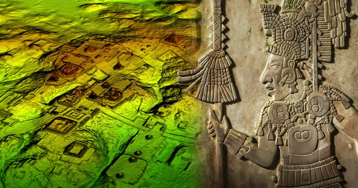
Airborne laser sensors firing pulses at rates exceeding 400,000 per second can now map cities beneath triple-canopy rainforest where traditional survey crews would require decades. Maya lidar surveys conducted across the lowlands of Guatemala and Belize since 2009 have revealed more than 60,000 structures by recording the time each pulse takes to return from the ground after penetrating gaps in foliage. The laser beam reflects from leaves, branches, and finally the forest floor, creating multiple returns that software algorithms classify into vegetation and bare-earth points. From those ground points, archaeologists generate digital terrain models showing causeways, terraces, platforms, and reservoirs built between 250 and 1000 AD.
Regional projects flown over Petén, the Mirador Basin, and Caracol document settlement densities, defensive networks, and agricultural modifications invisible from surface survey. The resulting bare-earth maps guide excavation teams to test features identified in the point cloud. Ceramic sherds and radiocarbon samples then tie detected architecture to Late Preclassic through Terminal Classic phases, confirming that platforms visible in the terrain model supported households occupied before collapse around 950 AD.
Maya Lowlands and the Problem of Mapping Cities under Jungle Canopy
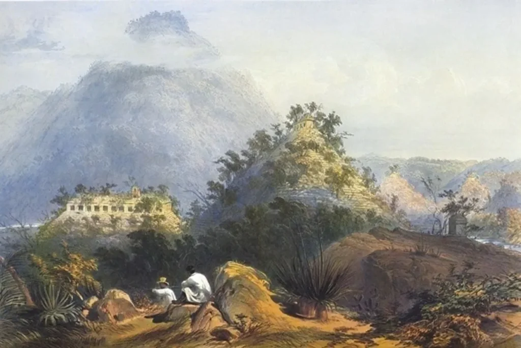
The Maya lowlands extend across northern Guatemala, Belize, and portions of Mexico where seasonal rainfall exceeds 1,500 millimeters and supports broadleaf evergreen forest. Canopy height averages 25 to 35 meters with emergent trees reaching 40 meters, blocking visibility of ground features from aerial photography and satellite imagery. Traditional archaeological survey required foot transects through undergrowth, recording each mound and structure by compass and tape measure. A single 100-square-kilometer zone might demand five field seasons and never achieve complete coverage due to terrain, property access, and dense vegetation masking low platforms.
Maya cities occupied these forested zones continuously from Middle Preclassic times through Terminal Classic abandonment around 950 AD. Urban cores featured pyramid temples, palace complexes, and ballcourts, while residential groups spread across kilometers of hinterland connected by raised causeways the Maya called sacbeob. Agricultural terraces, reservoirs known as aguadas, and defensive walls modified entire watersheds. Surface survey captured monumental architecture but underestimated total settlement extent and landscape engineering, leaving questions about population density, regional integration, and subsistence systems unresolved until lidar archaeology provided complete coverage.
What LiDAR Is: Pulses, Wavelength, Returns, and Canopy Penetration
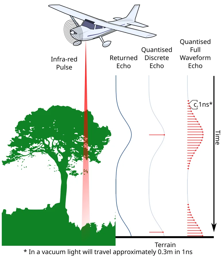
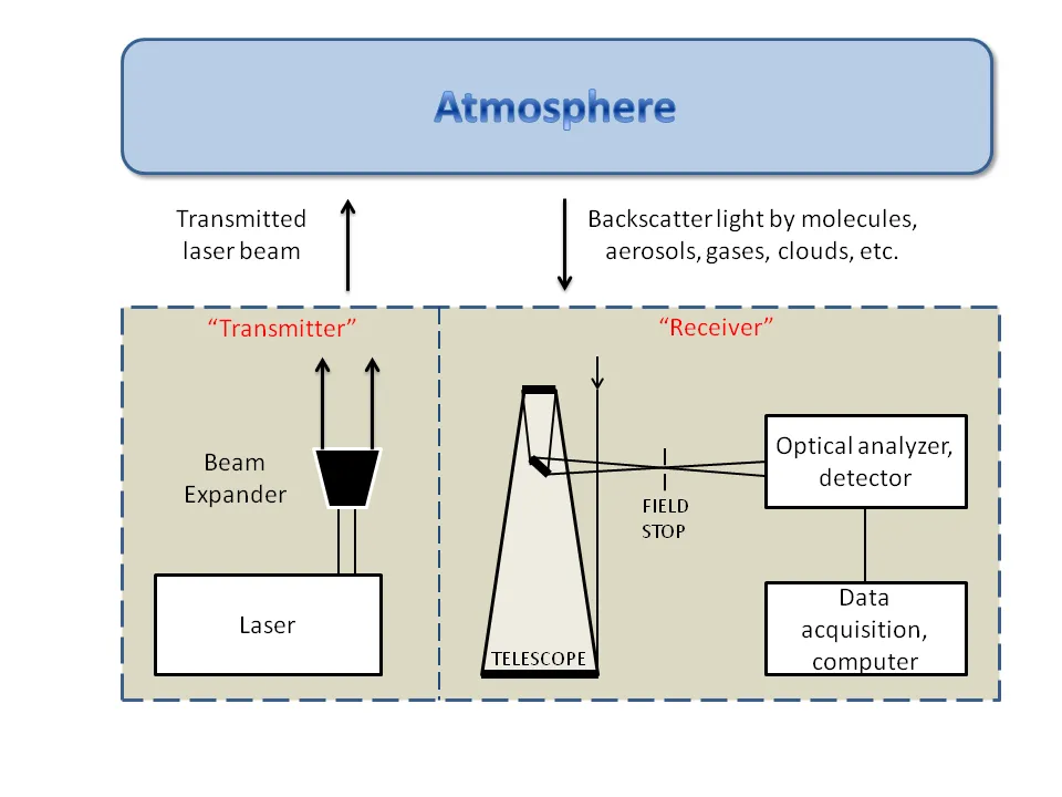
LiDAR, an acronym for Light Detection and Ranging, measures distance by emitting a focused laser pulse and recording the elapsed time until the reflected light returns to a sensor. Airborne systems mount the laser scanner, a GPS receiver, and an inertial measurement unit in a single pod carried beneath fixed-wing aircraft or helicopters. The laser operates at near-infrared wavelengths, typically 1064 nanometers or 1550 nanometers, which reflect strongly from both foliage and ground surfaces. Each pulse travels at the speed of light; the sensor calculates distance by multiplying the two-way travel time by light speed and dividing by two.
Jungle canopy does not form a solid barrier but consists of leaves, branches, and gaps through which laser pulses penetrate. A single outgoing pulse may generate multiple returns: the first from the canopy top, intermediate returns from mid-story vegetation, and a final return from the ground. Modern systems record up to four returns per pulse, storing each as a three-dimensional point with X, Y, and Z coordinates plus an intensity value indicating reflectance strength. The collection of millions of points forms a point cloud representing every surface the laser encountered, from treetops to forest floor, enabling lidar mapping of structures obscured by the jungle canopy.
Aircraft, Sensors, and Flight Parameters: Altitude, Scan Angle, Pulse Density
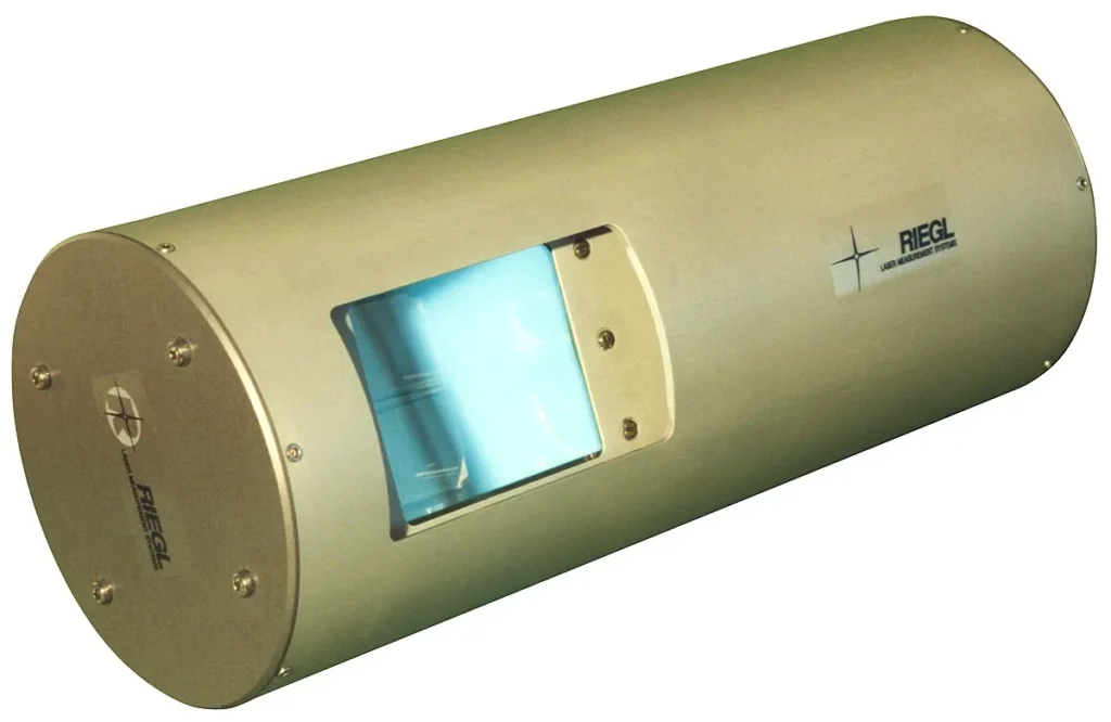
Lidar mapping of Maya cities employs twin-engine aircraft flying at altitudes between 500 and 900 meters above ground level, balancing swath width against point density. The lidar instrument sits in a belly mount and scans perpendicular to the flight path using an oscillating mirror that sweeps the laser beam across a strip beneath the plane. Scan angles range from ±28 to ±30 degrees from nadir, defining a swath width of roughly 600 meters at 600-meter altitude. Flight lines overlap by 50 percent so the edge of one swath covers the center of the adjacent pass, ensuring uniform coverage and eliminating gaps.
Pulse repetition frequency, measured in kilohertz, determines how many laser shots the sensor emits per second. Multi-channel systems fire three beams simultaneously at 150 or 175 kilohertz per channel, yielding combined rates of 450 to 525 kHz. At a ground speed of 70 meters per second and 25-hertz mirror oscillation, the instrument achieves point densities of 20 to 24 pulses per square meter on the ground. Dense canopy reduces the number of ground returns because some pulses never penetrate to the forest floor, but overlapping flight lines compensate by increasing the probability that at least one beam finds a gap above each spot.
Flight planning divides large survey areas into blocks flown over multiple days, weather permitting. Clouds, rain, and high winds halt operations because water droplets scatter the laser and turbulence degrades GPS positioning accuracy. Survey missions over the Petén region of Guatemala and the Puuc hills of Yucatán collected data during the dry season when cloud cover is minimal and foliage somewhat reduced.
From Point Cloud to Bare-Earth: Classification, DSM/DTM, and CHM
Raw lidar data arrives as billions of unclassified points recording every surface the laser touched. Processing begins with noise filtering to remove errant points caused by birds, low clouds, or sensor errors. Software then classifies each point into categories: ground, vegetation, building, water, or unassigned. Ground classification algorithms analyze local neighborhoods, identifying points that form the lowest continuous surface and flagging higher points as non-ground. Automated routines achieve 85 to 90 percent accuracy; human operators refine the results by inspecting cross-sections and manually reclassifying misidentified points.
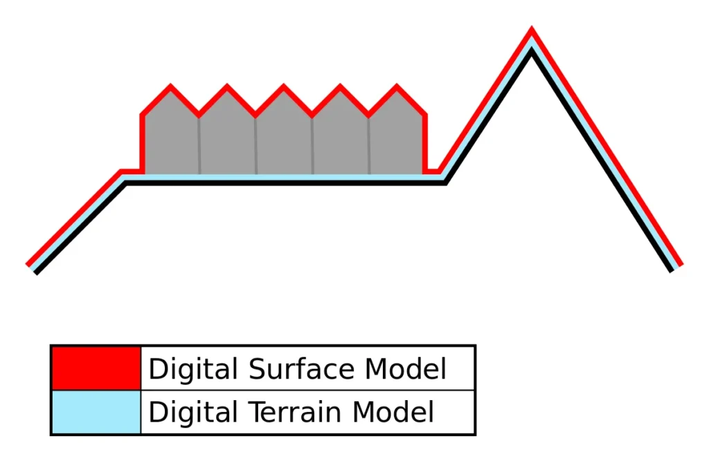
From classified points, the processor generates three primary elevation models:
- Digital Surface Model (DSM) interpolates a raster grid from first returns, representing the top of the canopy and any structures
- Digital Terrain Model (DTM) interpolates only ground-classified points to show the bare-earth surface
- Canopy Height Model (CHM) results from subtracting the DTM from the DSM, displaying vegetation and structure heights above ground
For lidar archaeology of Maya sites, the DTM is the critical product because ancient platforms, terraces, and walls appear as subtle elevation changes in the bare-earth surface invisible in the DSM where modern trees dominate. Processors export the DTM as a raster with node spacing of 50 centimeters to 1 meter, preserving fine detail while keeping file sizes manageable. Vertical accuracy depends on point density, terrain slope, and vegetation penetration. Studies comparing lidar-derived elevations to GPS-surveyed ground control points report root mean square errors of 10 to 15 centimeters in open areas and 20 to 30 centimeters under forest.
Visualizations That Reveal Sites: Hillshade, Local Relief, Sky-View Factor
Elevation alone can obscure archaeological features because regional slopes and large-scale topography dominate the visual range. Archaeologists apply visualization techniques that enhance local relief and suppress broad trends. Hillshade, the most common method, simulates illumination from a specified sun angle, casting shadows that highlight slope breaks and ridges. Varying the azimuth and altitude of the simulated light source reveals features oriented in different directions; a composite combining multiple azimuths prevents directional bias.
Local relief models filter the DTM into two components: a broad regional trend and fine-scale deviations. Subtracting the smoothed trend surface from the original DTM leaves a residual that emphasizes meter-scale bumps and depressions such as house platforms or quarry pits. The radius of the smoothing filter determines which features appear; radii of 5 to 20 meters suit Maya residential mounds, while 50-meter radii highlight larger plazas and pyramids.
Sky-view factor calculates the proportion of the sky hemisphere visible from each point, simulating diffuse illumination rather than a single light source. Depressions such as ditches or borrow pits score low because surrounding terrain blocks the view; ridges and platform tops score high. Sky-view factor reveals subtle earthworks in flat terrain where hillshade fails, and archaeologists working in the Maya lowlands often combine hillshade, local relief, and sky-view factor into red-green-blue composite images where different feature types stand out in distinct colors.
Built out of a love for history, kept free from distractions.
Spoken Past is an independent project shaped by curiosity, care, and long hours of research. Reader support helps keep it maintained, carefully researched, and open to everyone.
Features Detected in Maya Landscapes: Causeways, Terraces, Reservoirs, Walls
Raised causeways, known by their Yucatec Maya name sacbeob (singular sacbe), appear in lidar data as linear ridges 5 to 10 meters wide and 0.5 to 2 meters high connecting ceremonial precincts to outlying groups. The Maya constructed sacbeob by quarrying limestone bedrock and piling rubble into roadbeds surfaced with white marl. Maya lidar captures these features even when buried under 30 centimeters of soil and overgrown by trees, because the roadbed remains elevated above surrounding terrain. At Caracol, the DTM revealed a dendritic network of causeways radiating from the site core across 200 square kilometers.
Agricultural terraces cover hillsides throughout the southern lowlands, where the Maya built stone retention walls perpendicular to slope to create level planting surfaces. Terrace risers 0.3 to 1 meter high appear in the bare-earth model as closely spaced contour lines, often covering 70 to 80 percent of surveyed landscapes. Lidar mapping distinguishes terraces from natural slope breaks by their regular spacing, parallel alignment, and extension across multiple contour intervals.
Reservoirs and aguadas, depressions that collected rainwater for dry-season use, register as enclosed low areas in the DTM. The Maya excavated basins and lined them with clay to reduce seepage, creating water storage systems essential for supporting urban populations in a region lacking perennial streams. Defensive ditches and walls, particularly common around Terminal Classic centers facing external threats, show as linear depressions backed by elevated berms. The fortifications encircle hilltops or block access routes, demonstrating concern for security in the centuries before collapse.
Ground-Truthing After LiDAR: Survey Teams, Test Pits, Accuracy Rates
Maya lidar mapping identifies thousands of potential features, but confirming their cultural origin and function requires ground verification. Archaeologists prioritize high-probability targets, such as rectangular platforms clustered around plazas, and organize field seasons to visit, photograph, measure, and test-excavate representative samples. GPS units guide teams to coordinates extracted from the DTM; on arrival, crews describe visible architecture, record dimensions, and collect surface artifacts for preliminary dating.
Test pits excavated into platforms and terraces expose construction fill, floors, and deposits containing pottery sherds and charcoal. Ceramic typology assigns the sherds to established chronological phases, while radiocarbon dating of charcoal provides absolute age ranges. A 2023 study at Tikal tested 220 structures first identified in lidar data and found that 93 percent were accurately classified as residential platforms, confirming that automated feature detection achieves high reliability.
Ground-truthing also reveals features the DTM missed. Low structures on flat terrain may lack sufficient relief to distinguish from natural micro-topography. Looters’ trenches, modern logging roads, and limestone bedrock outcrops can mimic ancient construction in the bare-earth model. Experienced survey teams learn to recognize ambiguous signatures and adjust field strategies, verifying high-confidence features quickly and devoting more time to anomalies requiring excavation to resolve.
Dating What LiDAR Sees: Tying Features to Phases ≤ 1000 AD
LiDAR visualizations display topography without inherent chronological information; archaeologists must correlate detected features with established ceramic sequences and radiocarbon chronologies. The Maya lowlands use a phase system dividing the long occupation into Preclassic (2000 BC to 250 AD), Classic (250 to 950 AD), and Postclassic (950 to 1500 AD) periods, with finer subdivisions within each. Most mapped settlement dates to the Late Classic (600 to 800 AD) and Terminal Classic (800 to 950 AD), when population peaked before the southern lowland collapse.
Excavation into platforms and terraces recovers pottery styles diagnostic of construction phases. Late Classic polychrome vessels and Terminal Classic fine orange wares provide decade-scale resolution, demonstrating that many causeways, reservoirs, and defensive works were built or modified in the final centuries before abandonment. Radiocarbon dates on charcoal from construction fill and sealed deposits bracket building episodes; for example, terraces at Caracol yielded charcoal dated between 680 and 880 AD, confirming intensive landscape modification during the Late to Terminal Classic transition.
Stratigraphy within aguadas and wetland fields documents environmental changes through sediment cores. Pollen, phytoliths, and carbon isotopes indicate agricultural intensity, deforestation, and drought events that correlate with construction phases visible in the lidar data. By 950 AD, most southern lowland centers were abandoned; maya lidar surveys capture the settlement pattern frozen at that moment, with later Postclassic occupation sparse except in northern Yucatán.
Limits and Errors: Occlusion, Misclassification, and False Positives
Dense canopy occludes some ground areas despite overlapping flight lines; if no laser pulse penetrates the foliage above a particular square meter, the DTM at that location interpolates elevations from surrounding points, potentially smoothing over small features. Occlusion rates vary with canopy density, flight parameters, and season. Studies report ground point densities ranging from 1 to 10 points per square meter after classification, compared to the 20 to 24 total pulses per square meter emitted. The 50 to 75 percent reduction reflects jungle canopy interception.
Automated ground classification algorithms occasionally misidentify low vegetation, fallen logs, or limestone bedrock as ground, introducing bumps and pits into the DTM that mimic cultural features. Human review catches many errors, but subtle misclassifications persist, particularly in karst terrain where exposed bedrock and natural solution pits resemble quarries or storage features. Archaeologists develop interpretive experience distinguishing geological from anthropogenic signatures: rectangular shapes, alignment with other structures, and association with artifact scatters favor cultural origin.
Processing artifacts arise from flight-line boundaries, GPS errors, and interpolation across data gaps. Seams between adjacent swaths can introduce artificial elevation steps if the two point clouds are not perfectly aligned. Vegetation movement during the seconds-long interval between overlapping passes creates phantom offsets. Quality control procedures identify and correct these errors, but residual noise remains, especially in areas surveyed under marginal weather conditions.
What LiDAR Changes in Maya Urbanism: Density, Networks, and Regional Planning
Lidar archaeology surveys overturned assumptions about Maya settlement by revealing urban sprawl previously underestimated by ground survey. At Caracol, the DTM documented 5,000 structures across 200 square kilometers, implying peak populations exceeding 100,000, far above earlier estimates. The density of residential platforms, spacing of plazas, and extent of terracing demonstrated that Classic maya cities were not ceremonial centers surrounded by empty forest but continuously occupied landscapes integrating monumental and domestic architecture.
Regional coverage showed that sacbe networks connected centers into hierarchical systems. Causeways linked secondary sites to regional capitals, facilitating administrative control and economic exchange. The road systems, combined with defensive walls around certain centers, revealed political territories and evidence of competition or conflict during the Terminal Classic. Settlement clustering around elite residential groups, detected by mapping vaulted masonry structures that concentrate near plazas, indicated neighborhood organization and social stratification embedded in spatial layout.
Agricultural infrastructure visible in the bare-earth models transformed understanding of subsistence. Terrace coverage on 70 to 80 percent of some landscapes implied intensive cultivation supporting population densities approaching modern rural levels. Wetland field systems, aguada networks, and canals demonstrated sophisticated water management integrating urban, residential, and agricultural zones into planned regional economies active from Late Preclassic establishment through Terminal Classic collapse. Maya lidar technology continues to reshape archaeological interpretation by providing complete regional datasets that reveal connections between urbanism, agriculture, and political organization across the lowlands before 1000 AD.